N.A.Kozyrev’s causal mechanics seen
by an orthodox physicist
B. N. Chigarev
1. Introduction
N.A.Kozyrev, the famous Soviet physicist, worked at the problem of distant influence of irreversible processes on physical systems. His works in this field are important for the understanding of the “time” phenomena.
His works are valuable, at least, because he discovered volcanic activity on the Moon (Kozyrev 1963) and worked out a new method of trigonometric parallaxes determination based on measurement of difference between the true and seen star positions (Kozyrev, Nasonov 1978).
His first work was officially recognised in 1969, when the State Committee for Discoveries and Inventions awarded him a diploma for discovering volcanic activity on the Moon. The international Astronomy Academy awarded the Gold Medal to him in 1970.
His second work was experimentally verified in investigations, carried out by a group of researchers at the Institute of Mathematics of the Siberia Branch of the USSR Academy of Sciences. The results have partly been published in Doklady AN SSSR (the Reports of the USSR Academy of Sciences) during 1990-1991 (Lavrentyev et.al. 1990a, 1990b, 1991).
On the face of it, phenomena noticed by Kozyrev have no agreement with conventional models of contemporary physics. Furthermore, they are explained with the aid of “Causal Mechanics” proposed by Kozyrev himself.
However, having acquainted with Kozyrev’s works during the Moscow State University Seminar “Time Phenomena Investigation”, held in 1990-1991, the author of this writing was prompted to try to explain Kozyrev’s works from positions of the orthodox physics, even if this explanation is not comprehensive.
2. Analysis of principles of causal mechanics
Let us make an attempt to consider “Causal Mechanics” (Kozyrev 1963) from the position of general physics.
1. Kozyrev states: “A consequence follows a cause. Between these there is always a time gap” (Kozyrev 1963, p.97). According to the theory of relativity, an event, which is a cause, always precedes an event, which is a consequence. This happens in all frames of reference. If we take dx as a difference between cause and consequence coordinates, and dt as a corresponding time gap in a stationary frame of reference, then in a frame of reference moving along x direction at a constant speed v we have the following expression for the time gap dtў:
![]() ;
;
sgn(dtґ) = sgn(dt),
hence an event being a cause precedes an event being a consequence in all the frames of reference.
2. “Causal Mechanics” has got the following axiom: “ ... a cause and a consequence are always divided in space. Therefore, there is always an infinitesimal, though not zero, space gap dx between them ...” (Kozyrev 1963, p.97). This one and the analogous axiom concerning time gap dt are in agreement with the Heisenberg uncertainty principle. It lays down principal limitations on the possibility of measuring various physical magnitudes. Therefore, there is no basis to speak about dt and dx approaching zero (dxЧ dp іh; dEЧ dt іh) if we consider cause-consequence interaction in the frames of the orthodox physics (Landau, Lifshits 1972b).
Moreover, the fact that the speed of light is finite lays down additional limitations. L.D. Landau (1972b) showed that the inequality dpЧ dx і h can be considered as the relation (vў-v)dpЧ dt і h, where: dp — the uncertainty of measurement of a particle impulse during the measurement time dt; v (vў) — the speed before (after) measurement; (vў-v)dt — the particle position uncertainty.
According to (Landau, Lifshits 1972b) the difference (vў-v) is not allowed to be greater than c. Therefore, we can get the inequality dpЧ dt і h/c that shows impossibility of measuring impulse magnitude however fast and exactly.
Taking into account dp Ј mc, the minimum error in a coordinate measurement is:
d
x і h/mc.Thus a natural limitation on a particle localisation is introduced.
Let e.g. 2 electrons be approaching each other. Then, the maximum of their interaction energy uncertainty with the limitation on their localisation is:
d
E = e2/dx.Then,
d
tЧ dE і h; dtЧ e2/dx і h; dx/dt Ј e2/h.Thus we get a limitation on the ratio dx/dt proposed by Kozyrev.
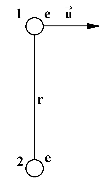
Fig.1. The influence of a charged particle (1), which is moving at the speed U, on the fixed charge.
3. Most of the phenomena which appear when macroscopic objects interact under laboratory conditions have electromagnetic nature. For this reason let us turn once again to the test particle interaction (Fig.1).
The force of electrostatic interaction is
F = e2/r2.
However, the charge e moving at the speed u also creates at the point 2 the magnetic field:
H = ue/cr2.
This field will interact with the electron magnetic moment mb giving additional energy to it:
![]()
and transferring mechanical moment projection h/2 along the axis which is parallel to H, and which simultaneously is the instantaneous axis of rotation of particle 1 with respect to particle 2.
Magnetic field does not transfer any additional impulse while the additional energy is proportional to ![]() lk, as Kozyrev has it proportional to
lk, as Kozyrev has it proportional to ![]() .
.
It should be mentioned that in the above estimation additional energy is involved, while Kozyrev claimed the existence of an additional force. However, first, such a force is not measured in any of Kozyrev’s experiments. He measured impact of dissipative processes on mass measurement, Beckmann thermometer readings, additional dynamic deviations in a vibration scales readings, free falling body deflection to the South, star impact on a resistor, etc. Second, it is not worth introducing an additional force, which does not transfer an impulse, but which changes internal energy and mechanical moment projection of the system (Kozyrev 1963, p.101). It is easier to use additional internal energy and angular momentum, which can be transferred to the body from e.g. magnetic field.
Physicists define such notion as “gyroscopic forces”. Such forces depend on the velocity and the sum of their works is equal to zero. For example, the Coriolis force ![]() and the Lorentz force
and the Lorentz force ![]() are gyroscopic forces.
are gyroscopic forces.
Many of Kozyrev’s experiments used motion with acceleration in an accelerated frame of reference, i.e. when v is not a constant (e.g. vibration). This results in an additional connection among the degrees of freedom through the forces of inertia.
The existence of the magnetic field and angular momentum interconnection at the macroscopic level was shown in 1915 by Einstein and de Haas. They proved that the spin magnetic moment is responsible for ferromagnetism in metal by demonstrating the rotation of an iron cylinder with a coil placed around it suspended on a thin thread. The reverse effect of the magnetisation of an iron rod affected by its fast rotation was shown in 1909 by S.Barret.
However, we cannot claim to explain all the Kozyrev’s effects by these phenomena. Kozyrev found effects, possibly of various nature, which are of the order of 10-3-10-4% of the measured magnitude. It is difficult to imagine how we can use the main postulates of “Causal Mechanics” to explain the effects of influence of acetone evaporation on the Beckmann’s mercury thermometer readings, as it is not clear how “the rotation of the cause with respect to the consequence” occurs, and where the angular momentum is transferred to.
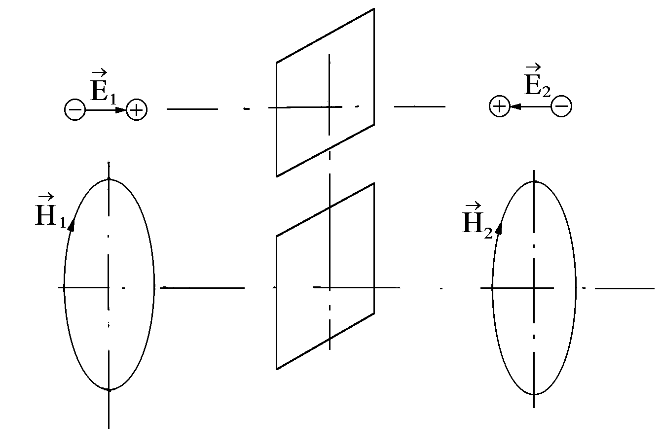
Fig.2. The difference of the nature of electric and magnetic fields. When reflecting the axial vector from the plane (![]() ), but (
), but (![]() ). When reversing the time (t
). When reversing the time (t
4. To describe the impact of the cause on the consequence Kozyrev used a “pseudovector” (axial vector) and realized the reason for the irreversibility of the “time flow”. The difference between a vector and a pseudovector, when the time is reverse, is well known in physics. As an example we can take the comparison of the nature of electric and magnetic fields (Fig.2). When the axial vector ![]() reflects from a mirror
reflects from a mirror ![]() 1 =
1 = ![]() 2, but
2, but ![]() 1 = -
1 = -![]() 2. When the time is reversed (t®-t), the polar vector
2. When the time is reversed (t®-t), the polar vector ![]() does not change, but the axial vector
does not change, but the axial vector ![]() changes its sign as charges begin to move in the opposite direction.
changes its sign as charges begin to move in the opposite direction.
3. The analysis of experimental grounds for causal mechanics
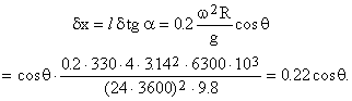
1. Kozyrev gave the example of deviation of a free fall trajectory from a vertical line in the meridian plane as the simplest experiment that confirms the axioms of “Causal Mechanics”. “... The height of the free fall was l = 158cm in these experiments. The displacement to the South was dlS = 4.4mm, the displacement to the East was dle = 28.4mm which is in a good agreement with the theory. Denoting dQp as the horizontal component of asymmetric forces in a moderate latitude, we then have:
![]()
hence
![]() = 2.8·10-5 at q = 48є.
= 2.8·10-5 at q = 48є.
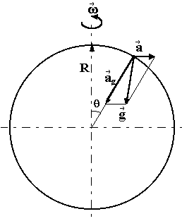
Fig.3. The forces impressed upon a free falling body in an accelerated frame of reference, which is connected with the Earth.
This value is in a good agreement with the above value of the gravity asymmetry.” (Kozyrev 1963, p.104)
Let us consider the results of this experiment from the point of view of the orthodox mechanics. In an accelerated frame of reference, taking the Earth rotation into consideration a body is under the influence of the gravitational force GMearthm/R2 and the centripetal force is mw2Rcosq (see Fig.3).
The mean acceleration of gravity g is the vector sum of the gravitational gMearth/R2 and the centripetal w2Rcosq accelerations. These values ratio defines the tangent of the angle of inclination t of the mean acceleration of gravity g in the meridian plane.
When the fall is free, this value changes because of the decrease in R. According to the Momentum Conservation Law the horizontal component of the speed does not change. Hence taking the small value of t into consideration, wR =const and w2R2 =const we have:
![]()
The additional displacement (dDS) in the meridian plane will be:
![]() m.
m.
Thus the simplest estimation of the value dDS agrees with the observed value.
2. The second-simplest Kozyrev’s experiment concerns vibration scales weighing. “In the experiment one load is rigidly hung on a wire, another load is hung on an elastic rubber or a spring. When the support vibrates, the scales end with a rigidly hung load remained practically steady. So the other scales end with the elastic hanging vibrated with an amplitude which was twice as much as that of the middle of the scales. It turned out that beginning from a certain vibrational acceleration the elastic hanging end of the scales shifts downward with an abrupt change ... at that moment the vibration acceleration of the hanger equal g at the frequency round 30Hz. ...The step value is about 31mg per kg, i.e. 3.1·10-5...” (Kozyrev 1963, 1963, p.108)
2.1. It should be noted that the step-like change in the scales readings cannot be inferred from the main equation of the “Causal Mechanics” by Kozyrev, i.e. it cannot be regarded as its experimental confirmation.
2.2. The Kozyrev’s effects occur when the acceleration at the fixation point (ab) of the elastic hanger approximately equals g (Kozyrev 1963, see Fig.1).
2.3. If ab і g, the symmetry of vibrating lever impact on the elastically hung load is broken. When moving up, the vibrating lever will be under the action of inertia forces, which are transferred from the load through the elastic hanger. When moving down, the lever cannot cause load acceleration. The load simply falls with the acceleration g. Elastic hanger may smooth and complicate load motion in comparison with the case when the load is hung with an inelastic thread. Physicists consider those similar to the above problems as Fermi acceleration problems (Sagdeev, Zaslavsky 1988).
The simplest model in this case is the one with a ball jumping on a vibrating platform. This problem has been thoroughly examined by P.J.Holmes (1982). Results of his experiments can be found in (Tuffilaro, Abbanoa 1986).
If an impulse is transferred from the platform to the ball instantly, then we have difference equations:
![]()
here tn is the impact time, dP/m is the wall transferred impulse divided by the mass, hn is the height of the ball jumps.
The problem is asymmetric because when the ball and the platform are moving in the same direction at the moment of the jump, an average time between 2 successive jumps is less than in the case when their directions are opposite.
Different phenomena can be observed in similar environment: chaotic vibrations, subharmonic appearance, etc. Concerning Kozyrev’s experiments, a step change in a load average position, when the frequency of forcing vibrations wfv is changing, is explained through a resonance corresponding to frequencies multiples of 1/T (T is the time between 2 jumps in the Holmes’s experiments or the time between 2 periods of free fall in the Kozyrev’s experiments). It should be mentioned that the problem is nonlinear, and t=t(wfv). The process is qualitatively depicted in Fig.4.
The reason for vibration asymmetry may be much simpler. Kozyrev used electromagnetic relay for vibration forcing. The hyroscope weighed 400g. The vibration amplitude was about 0.3mm. The frequency was approximately 30Hz. This is an oscillating system with a high inertia load. The relay oscillating displacement is asymmetric even without a load. That is why we have the system of coupled nonlinear vibrating systems, which parameters Kozyrev did not measure. At the same time, the measurements have been carried out with the accuracy as low as 10-3% of the measured magnitude. Not every control device can do that.
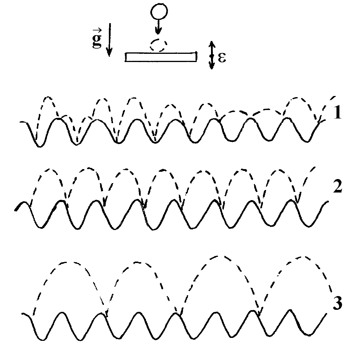
Fig.4. Jumping ball on a vibrating platform. 1 — chaotic motion; 2 — motion with frequency f = 1/T; 3 — motion with the frequency f < 1/T.
A general note should be made that in experiments similar to that of Kozyrev appearance of additional ways for energy dissipation can be regarded as an effective mass increase. The energy may start to dissipate due to e.g. a resonance appearance, an establishment through beating of connection between vibrating and rotating degrees of freedom, etc. Furthermore, additional connection may be caused by inertia forces that are proportional to acceleration, i.e. F = ma + Fdis(a).
Kozyrev claimed that by using a vibrating hangpoint he created a situation when a load is under the symmetric action of forces, while additional displacements are due to “asymmetric forces of the Earth rotation”. For example, “... in a thread-hung gyroscope experiment the gyroscope turned out to have additional displacement when its axis is along the meridian. This displacement is obviously connected with Earth asymmetric forces. If vibrations are introduced, then the displacement of the order of 0.06mm towards the North is observed (the pendulum length is 330mm). This effect is not dependent on the gyroscope rotation speed and it can be observed if any thread-hung unrotating object is vibrating” (Kozyrev 1963, 1963, p.107). In such a situation the hung object is not symmetrically forced as well, since the vertical projection of the thread strain is m(g-a) if the motion is down, and m(g+a), if up.
Let a be 0.1g. According to Fig.3, we have:
![]()
in the first case, and in the second case:
![]() .
.
This means that the displacement towards the North is
3. To make quantitative analysis of the more complex Kozyrev’s experiments is not easy to do because, first, the complete set of numerical characteristics of experimental set-ups is not known, and, second, Kozyrev’s schemes have many degrees of freedom and to make a detailed analysis numerical simulation is needed. However, the following should be mentioned:
sin x = x (1-x2/6+...) = x (1 -0.052/6+...) = x (1 -4·10-4+...)
and we have to take this nonlinearity into account. The same is with elastic hangers. It is unrealistic to expect a linearity of the order of more than 10-5 to be present in the Hook Law.
![]() .
.
If the force acts when V = 0, then the change is P2/2m.
4. Analysis of how the true star position influences physical systems
Kozyrev’s works contain description of a great number of interesting experiments. However to analyse and to reproduce those we would need to know in more details conditions of their accomplishment.
That is why we would dwell upon only one experiment, that is certainly of practical interest. It involves the problem of the true star position influence on physical systems (Kozyrev, Nasonov 1978).
1. As a basic concept for studying the star influence on physical systems Kozyrev uses the notion “time density”.
“The time density is a variable due to the fact that in different processes time can be either spent or generated. For this reason different phenomena may be interconnected even though they seem to have nothing in common. Every time, every place various processes are occurring. Therefore, changes in the time density must lead to changes of physical properties of matter that is close to the process. Experiments showed that these changes may involve elasticity, electroconductivity, photoeffect electron emittance, and even a body volume... . The time is not transmitted. In contrary it appears all over the Universe simultaneously... . The information can be transferred instantly to any place. The distance just makes this transfer weaker. As experiments show, it happens in accordance with an ordinary law, i.e. in inverse ration to the distance squared. ... The time action can, first, be shielded, and, second, be reflected, ... . The reflectance of an Al coating is about 50%. The time action can be substantially shielded from processes by a 1-cm plate of any solid high-density body. ... Changes in matter caused by absorption (of time, B.Ch.) can transmit so that time action transmittance along a solid conductor (a wire or a hose) become feasible” (Kozyrev, Nasonov 1978, p.171).
The true star position registration was carried out at the 5-meter reflector at the Crimea Astrophysics Observatory.
The sensor was the Wheatson bridge with 5.6kW metal-film resistors OMLT-0.125 having the 1.5·10-5 positive temperature index. The galvanometer division was 2·10-9A (R =5.6kW ). The bridge feed was the 30V stabilised voltage. The voltage had been switched on for an hour before the experiment started.
Kozyrev points out that “... the action had to be terminated very soon for 15-20 minutes were required to put the system into the original condition. Nevertheless, exact return had never been accomplished and the structure changes had been accumulating. That was why by the end of the night the system had lost its sensitivity, and it needed to be given a long rest for 1 or 2 days, or even removed from the housing, so that its sensitivity recover. The system sensitivity was measured through acetone evaporation impact on the resistivity. When space objects were observed, the galvanometer needle was deflected in the same direction” (Kozyrev, Nasonov 1978, p.175).
Let us analyse Kozyrev’s set-up characteristics. Power dissipated in a resistor:
![]() W.
W.
Resistor surface area:
S =pDL =3.14·1.2·7 =26.4mm2.
Power dissipated at the surface unit:
P = W/S = 0.16/26.4Ч 10-6W/m2.
For comparison: the sun constant is 1.36·103W/m2.
We could hardly expect the star impact intensity to be of this order. An increased convective heat transfer seems to be more real cause for the resistivity decrease. The fact that in Kozyrev’s experiments the working resistor was covered with a paper hood, moved forward and placed after the spectrometer aperture just enhances the Wheatstone bridge sensitivity to the convective heat transfer. Since, first, the paper shield results in stronger working resistor heating than the others’. Second, it introduces a time delay in the resistor reaction to convective heat transfer variations.
It is also possible, that large quantity of Aluminium connected to the bridge serves as a radiator being the bar for other resistor temperature stabilisation.
The Cu heat transfer index is 389.6W/m K, while the air heat transfer index under the normal conditions is 257·10-4W/m K, namely 4 times lower. Hence, heat transfer along the wires connecting the bridge resistor must be playing an essential role in stabilising the temperature.
Let us make an estimation of the temperature phenomena in the bridge that Kozyrev used.
The increase in the temperature related to the bridge heating is:
d
T =where cAl = 900J/kg K is the Al heat capacity, (for Cu — 396J/kg K; for an assessment this is not critical), V = 7.9·10-9m3 is the resistor volume, r = 2.4·103kg/m3, t1 = t2/600sec is the characteristic resistor heating time.
Kozyrev points out that heating lasted even more than t2 і 1 hour. But since we do not take into account heat losses in the above estimation, we take t1 = t2/600.
The resistance change at such heating is
d
R/R = aЧ dT = 5.6·10-3,where a =10-4K is the resistance temperature index (Kozyrev, Nasonov 1978).
This is 102-103 times more than the resistance change caused by star impact on the resistor (dR = -106Rnom). On the other hand, to lower resistor heating by 0.01 or 0.001 through convective heat transfer intensity increase is rather feasible. In this case the resistance will decrease. Kozyrev observed this decrease at both the star impact on the resistor and the acetone evaporation from the wool.
It should be mentioned that the convection increase may be caused by a variety of processes, including a short-time heating. Moreover, in some cases initial effect may be enhanced by introducing a convective instability. Observing effects of the order of 10-3-10-4% of the magnitude, we should take into consideration that a resistor noise EMF is close to 1mV/V, and that metal soldered joint heating may cause a thermoEMF. For example, a Cu/Al thermoelectrical couple has at emf = 3.4mV/K. Kozyrev has not analysed such problems.
The next group of problems deals with electrostatic charge appearance on the rigid body surface.
It is known that there are no ideal solid isolators. They always contain structural defects. This results in a nonzero total internal charge of a solid state. Accompanying this electric field is compensated by ions, present in the air. Electron emission is also creating a double electrical layer on a metal surface that leads to a contact voltage. The presence of double layers on a solid body surface makes changes in an electron density distribution along the conductor depth (Kittel 1978):
n(r) - n0 = ![]() ,
,
where ef is the Fermi energy, U(r) is the potential distribution along the cross-section, n(r)-n0 is the electron concentration deviation from the homogeneous distribution.
The shielding depth for metals is 1Е. Kozyrev used metal-film resistors. Let us take the film depth of an order of 1
mm, Then l/d ratio is 10-4. Kozyrev’s effects are of the order of 10-3-10-4 % of a nominal value, and an n(r) unevenness cannot be neglected. The concentration n(r) determines the metal thermoconductivity. That is why polarisation phenomena may influence both heat transfer and film electroconductivity. There are also some indirect evidence on possible importance of electrostatic changes in Kozyrev’s experiments.So, Kozyrev claims that “time action transfer ... along a hose becomes possible” (Kozyrev, Nasonov 1978). At the same time it is known that even in 1730 Gray managed to transmit a charge for several hundreds of feet along a rope hung on thin threads (Filonovich 1990).
Kozyrev points out further that the sensor should be placed on as thin fastenings as possible, that its parameters change during the work, that for the sensitivity to recover 1 or 2 days are needed, and sometimes even the sensor need to be removed from the cover. As Kronfeld showed (According to (Filonovich 1990)), the time constant of a charge decrease of a friction electrified isolator is approximately 60min. If the electrified sample remains in a small closed camera, it keeps its charge for several weeks.
Kozyrev’ use of a asymmetric torsion scales as a sensor may serve as an indirect evidence of importance of electrostatics and convection. Since Lebedev’s time it is known that the main obstacle for work with torsion pendulum are electrostatic fields, convective streams and radiometric action determined by the fact that gas molecules are reflected from a warm side with a higher speed than from a cold one (Landsberg 1976). The work (Aleksandrov 1991) has an evidence that torsion pendulum has not worked in the vacuum in the Kozyrev’s experiments.
2. The principal Kozyrev’s argument is the claim that the orthodox physics is unable to explain the true star position impact on physical systems. Let us show that it is not quite so.
It is known that potentials of the field created by moving point charges are (Feynman et.al.1964):
 (1)
(1)
These are called Lienar-Vikhert potentials. Here ![]() is the radius-vector from the point of the charge location to the point of observation, and other values in the right sides of the equalities are taken at the time delay moment:
is the radius-vector from the point of the charge location to the point of observation, and other values in the right sides of the equalities are taken at the time delay moment:
tў = t - R(tў)/c.
From Eq.1 we can see that at the charge trajectories where acceleration is small, the delay time R(tў)/c is practically compensated by the amendment ![]() , i.e. (
, i.e. (![]() )late ~ Rs. R.Feynman said: “... a late Coulomb field requires an amendment, which equals the rate of change of the late Coulomb field multiplied by R'/c selflateness” (Feynman et.al. 1964).
)late ~ Rs. R.Feynman said: “... a late Coulomb field requires an amendment, which equals the rate of change of the late Coulomb field multiplied by R'/c selflateness” (Feynman et.al. 1964).
From Eq.1 we may derive the fields ![]() and
and ![]() (Landau, Lifshits 1972a):
(Landau, Lifshits 1972a):
 ,
,
![]() . (2)
. (2)
Electromagnetic field consists of 2 parts; the first term depends only on the charged particle speed and at long distances decreases proportional to 1/R2 . The second term depends on the acceleration and decreases proportional to 1/R.
Furthermore, we usually make the assertion that the first term should be neglected and only the radiation caused by the charge acceleration should be considered. However, taking into account that Kozyrev dealt with small amendments to the measured values (~10-6), pay attention to the following: the electromagnetic radiation (the second term in Eq.2) interacts with various substances and causes effects proportional to the absorbed energy, i.e. eE2rad ~ 1/R2 , which are hard to observe.
On the other hand, the magnetic field, which depends only on the speed of a charged particle (the first term in Eq.1), and is proportional to 1/R2 as well, will influence the magnetic moments of electrons (or nuclei?) bringing a perturbation with the energy Hm, where m is the magnetic moment magnitude. This perturbation magnitude will be proportional to 1/R2 as well.
Let us estimate the ratio of these perturbation energies (Hm)st/(eE2)rad for a single electron.
The equation of a free electron motion is:
![]() .
.
Let E=E0e-iwt, then
-w
2mX = -eE0; V = Xw0 = eE/mw.The kinetic energy Tkin of an electron in the field E0e-iwt is:
Tkin = mV2/2 = e2![]() /2mw2.
/2mw2.
The potential energy of an electron in the magnetic field H is:
P = -ežH/2mc,
where mb = ež/2mc. Let us determine the ratio:
P/Tkin = (ež/2mc)H(2mw2/e2![]() ) = (ž/ce)(Hw2/
) = (ž/ce)(Hw2/![]() ). (3)
). (3)
Let us estimate the ratio H/![]() according to Eq.2. Considering v/c << 1 we get:
according to Eq.2. Considering v/c << 1 we get:
 (4)
(4)
from Eqs.3 and 4 it follows that:
here q = en, žc/e2 = a-1 = 137, K = ![]() .
.
The last term in Eq.5 depends on the ratio squared of the acceleration of the emitting and excited charges. From Eq.5, we can obtain the additional perturbation introduced by the magnetic field:
P = (V/c) 137 (K Tkin).
It is similar to the form proposed by Kozyrev:
dF
~ (V/c2)F0, c2 = c/137K.Influencing the electron spin, the magnetic field changes its potential energy and angular momentum projection on the axis H. The electron momentum does not change during this process.
As it is seen from the Lienar-Vikhert equations, this perturbation will seem to originate from the true position of the moving charge.
The existence of star magnetic fields is a well-known fact (Parker 1982). The cycles of their activity, flashes, the hot corona existence, etc. are the indirect evidences of star magnetic fields.
However, the direct impact of star magnetic fields on the measuring devices proposed by Kozyrev seems to be dubious. The disturbance of the Earth ionosphere and magnetosphere, or the disturbance of the gradient of potential of atmospheric electricity seems to be more probable. It is known that the voltage between the sea level and the 50km height is about 4·105V. And the electric field near the Earth Surface is 150-200V/m.
If we assume that standing waves originate in this gap (50km), then their frequencies would be in the kHz range. We also can assume the existence of additional modulation of the flux of charged particles by these longitudinal waves and the influence of these disturbances on a resistor. However, it is not easy to make acceptable estimations of the frequency range from Kozyrev’s experiments. Only indirect estimations are possible. So Kozyrev points out that the reflectance of a metal mirror is about 50%. Hence we deal with a low frequency radiation with the frequency w << s/e0, where s is the metal conductivity. Here the refractive index for low frequencies (Feynman et.al. 1977) is:
![]()
The real part of the refractive index n is equal to its imaginary part.
According to the estimation made by R.Feinmann (1977b), the “low frequency behaviour” of copper begins at w<<1012Hz. However the depth of the skin-layer will then be:
![]() =16.7·10-8m.
=16.7·10-8m.
Kozyrev observed the “time flux penetration (Kozyrev, Nasonov 1978) through the 0.5mm-thick Al plate, i.e. the frequency must be:
w
< 0.028(m2/s)/d2=112·103Hz.When Kozyrev closed the main mirror by an Al plate the effect decreased, though not much. This fact may serve as an indirect confirmation of such a great wavelength.
Let us assume that the perturbation is only 1/100 of the atmospheric electric field, i.e. it is equal to 1V/m. Then the density of the electromagnetic energy flux will be:
S = e0 E2 C = 12·3·108/(4p·8·109) = 2.65·10-3W/m2.
One should note that the specific dissipated power on the resistor surface is 6·103W/m2, i.e. 106 times greater than the supposed disturbance amplitude.
Therefore, the direct influence on the resistance seems improbable. Kozyrev also pointed out that the system is not always sensitive to the distant influence of dissipation processes, but it works only for a limited period of time.
The given estimations are admissible for the transverse component of an electromagnetic wave, when the wavelength is less than a characteristic size of the design. If we take into consideration the longitudinal component at great wavelengths, we must realise that both a shielding plate design and its earthing conditions are important. The description of the experiments has no such information.
If we assume that the effective absorption of electromagnetic energy of a certain frequency is possible not only in the volume of a rigid body but also in the “ion coat” near its surface, then taking into account small specific heat capacity of a gas (Cp=1.23kJ/m3·K for air) we would obtain a substantial temperature increase which changes the convective heat transfer conditions.
Let us assume that the depth of the “ion coat” d = 10-7m, then the temperature increases during 1s comes to :
d
T = S/Cp d = 2.65·10-3/(1.29·103·10-7) = 20K.In reality dT will be less as it is obvious that the characteristic heating time for this layer is less than 1s.
The perturbations near the resistor and the reflector may cause convection. The reflectance of the time flux is 50%, i.e. 50% of the time flux energy is absorbed by the reflector. Besides, the telescope tube creates the air column where the convection occurs. This very convection may influence the resistor heat transfer. The delay time in the response time of Kozyrev’s sensors may be explained by the fact that the development of convective streams and the heating of the system elements require some time. The indirect confirmation of this hypothesis is:
The above analysis cannot be considered as an answer for the mechanism of the effects, which Kozyrev observed. These are only some questions which must be answered before rejecting the orthodox physics and introducing new essences into consideration.
The experimental investigations on “the registration of the matter response to an external irreversible processes” (Lavrentyev et.al. 1991), “which are functionally connected with ... astrophysics experiments (Lavrentyev et.al.1990a, 1990b) and are their ideological and methodological basis”, cause many questions as well. For example, the weighing was performed with the help of analytical scales VLR-200 (the accuracy is 0.0001g).
“The investigation of human body processes impact on physical systems was done when an operator held an examined object with a build-in thermometer in hands for a certain time (8min, B.Ch.)” (Lavrentyev et.al.1991). But this contradicts the rules of handling scales (Kreshkov 1971) in items, which concern allowed touching of scales during their work and necessity of temperature stabilisation of a weighed object for accurate readings.
Another question arises when the Sun true position is analysed (Lavrentyev et.al. 1990b, p.368). The authors claim: “... The Sun has been chosen as an influencing body, for all known Sun impacts on Earth sensors are limited by the speed of light. For these impacts to reach the Earth 8.3min are needed. Correspondingly, the angle between the true and seen Sun positions is 2є4'.” In reality the angle is approximately:
t =
360· 8.3min/(364days· 24hours· 60min) = 0.0057єand the turning angle because of the Earth rotation is:
t
earth = 360· 8.3/(24·60) = 2.075є.It is not clear what impact was registered by the authors.
These are reasons for which even detailed experimental proof of the effects observed by Kozyrev may not eliminate their possible explanation from the viewpoint of the orthodox physics.
REFERENCES
ALEKSANDROV E. B. (1991). Nonsense. Poisk (Sweep). N.9(95) and N.10(96) (in Russian).
FEYNMAN R.P., LEIGHTON R.B. and SANDS M. (1964). The Feynman Lectures on Physics, V.2. New York.
FILONOVITCH S.R. (1990). The Fortune of the Classical Law. Moscow (in Russian).
HOLMES P.J. (1982). The dynamics of repeated impacts with a sinusoidally vibrating table. J. Sound and Vib, V.84, pp.173-186.
KITTEL Ch. (1968). Introduction to Solid State Physics. London, New York.
KOZYREV N.A. (1963). Causal mechanics and the possibility of the experimental research of time. In: History and Methodology of the Natural Sciences. N.2. Moscow, pp.95-113 (in Russian).
KOZYREV N.A. and NASONOV V.V.(1978). A new method of trigonometric parallaxes determination based on measurement of difference between the true and seen star positions. In: Problems on Research of Universe. Moscow, pp. 168-179 (in Russian).
KRESHKOV A.P. (1971). Foundation on Analytical Chemistry, V.2. Moscow (in Russian).
LANDAU L.D. and LIFSHITS E.M. (1972a). The Short Lectures on Theoretical Physics. Quantum Mechanics. Moscow (in Russian).
LANDAU L.D. and LIFSHITS E.M. (1972b). The Short Lectures on Theoretical Physics. Mechanics and Electrodynamics. Moscow (in Russian).
LANDSBERG G.S.(1976). Optics. Moscow (in Russian).
LAVRENTYEV M.M., YEGANOVA I.A., LUTSET M.K. and FOMINYKH S.F.(1990). Remote effect of stars on a resistor. Soviet Physics Doklady, V.35(19), pp.818-820.
LAVRENTYEV M.M., GUSEV V.A., YEGANOVA I.A., LUTSET M.K. and FOMINYKH S.F.(1990). Detection of the true position of the Sun. Soviet Physics Doklady, V.35(11), pp.957-959.
LAVRENTYEV M.M., YEGANOVA I.A., LUTSET M.K. and FOMINYKH S.F.(1991). Detection of the reaction of matter to an external irreversible process. Soviet Physics Doklady, V.36(3), pp.243-245.
MARTYNOV A.V. (1989). Confession Way. Moscow (in Russian).
MOON F.C.(1987). Chaotic Vibrations. An Introduction for Applied Scientists and Engineering. New York.
RUZMAIKIN A.A. (1990). Magnetic fields of stars. In: Encyclopaedia of Physics, V.2. Moscow (in Russian).
SAGDEEVR.Z. and ZASLAVSKY G.M. (1988). An Introduction to Nonlinear Physics. From Pendulum to Turbulence and Chaos. Moscow (in Russian).
TUFILLARO N.B. and ABBANO A.H. (1986). Chaotic dynamics of a bouncing ball. Am. J. Phys, V.54, N.10, pp.939-944.